Physics knows the constant c, the speed of light in a vacuum. Anyone who has approached this science cannot help but be fascinated by that value, which seems to contain within it the entire complexity of the Universe. Despite its simple formulation (299,792.458 kilometers per second), its implications for almost everything— from time dilation to gravity or the expansion of the Universe—make it difficult to grasp fully.

Economics, too, has a mysterious constant: the rate of return on capital (r). Economics is not physics, of course; and for r we cannot give an eternally immutable figure as we can for c. Yet it should surprise us that, over centuries, r has remained on average between 4% and 5%. Whether we look at eighteenth-century London, nineteenth-century Paris, or twentieth-century New York, we find that the average return on capital oscillates around those same percentages. It is not (on average—individual cases may vary widely) 1%, nor is it 15%; it is almost always between 4% and 5% (Th. Piketty, Capital in the Twenty-First Century, The Belknap Press of Harvard University, 2014, Kindle edition, location 8%).

Why is the rate of return on capital so constant? I do not think we have a clear explanation, but I will risk putting forward a hypothesis.

To introduce it, I suggest we step back to the time of the Roman Empire and focus on something that seems quite distant from our modern economy: the slave markets. How much was a slave worth in Rome? According to the sources available, in the first and second centuries CE, in Egypt, an ordinary slave might cost between 300 and 500 denarii—that is, between 90 and 150 grams of gold. To this purchase price one had to add food, lodging, and very little else. All of that might amount to roughly 100 denarii per year (about 30 grams of gold).

Thus, if one purchased a 15-year-old slave who remained productive for another 15 years (the life expectancy of slaves engaged in demanding labor rarely exceeded their early thirties, and beyond that age their performance likely declined), the total cost of that slave over a 15-year period would amount to between 1,800 and 2,000 denarii (roughly 540 to 600 grams of gold).

What return did the owner obtain from such a slave? The daily earnings of an unskilled free laborer were approximately 1 denarius. A slave working 270 days per year would therefore generate 4,050 denarii over 15 years. Those 270 days imply an almost continuous workload, with few days of rest (around 60 per year). In other words, an investment of 1,800–2,000 denarii would yield a profit of between 2,000 and 2,200 denarii over 15 years. That is, about 130 to 145 denarii per year—corresponding to an annual return of roughly 6.5% to 8%.

This is not the 4–5% typical of the modern era, but it does coincide with what appear to have been the returns on capital in the Roman Empire (between 6% and 8%, with 12% being the legal maximum). Interestingly, that 6.5–8% range aligns with the simple result of dividing the investment by the slave’s useful working life. If we assume that r ≈ 1/L, where L is the slave’s working life, then with L = 15 years we obtain r ≈ 6.7%, and with L = 12.5 years, r ≈ 8%. Life expectancy at birth in Rome was around 20–25 years, but anyone who reached adolescence could expect to live another 15–20 years, although the wear of manual labor meant that performance would decline after the age of 30. A working-life range of 12 to 15 years is therefore plausible.

In any case, these are averages; for an 18-year-old slave (perhaps the ideal age, since one might expect full adult productivity throughout those years), the purchase price would be higher, which would naturally adjust r back toward the relationship noted above (r ≈ 1/L). There is no need to go further here: the point is simply that it is not unreasonable to think that the return on capital embodied in a slave (purchase price plus maintenance costs) could be understood as a function of that capital and the slave’s useful working life.

It is as if the economic structure incorporated a temporal horizon determined by the duration of working life. From that horizon r would emerge. Put differently: the economy discounts human life.

If we now return to the familiar 4–5% with which we began, we can see that expressing it in relation to working life—not of the slave but of the modern worker—introduces a certain coherence. A 4% return corresponds to a working life of roughly 25 years; 5% to about 20 years. For the eighteenth or nineteenth centuries, these figures are not implausible. After the age of 40–45, many manual workers experienced a decline in effectiveness, not to mention illness, injury, or premature death. It is therefore not unreasonable to think that this seemingly constant rate of return might be linked to the length of people’s productive working lives.

Similarly, the slow decrease in returns observed over recent decades may be connected to the extension of fully productive working life—a working life that now begins later, closer to 25 than to 20, due to longer periods of education, and that extends beyond 50, whereas in an era dominated by manual labor that age already marked the end of full productivity. The point is not to be exact, but simply to underline that the useful life of the worker determines the order of magnitude of the rate of return.

Thus, as a provisional hypothesis (if the redundancy may be forgiven), we may suggest that the rate of return on capital is determined by the average useful length of working life. This would explain the higher returns observed in antiquity (when working lives were shorter) and the slow decline in the rate of return over the past century, linked to the gradual extension of working life—a working life that, as noted above, now begins later for most people than it did a hundred years ago (due to longer periods of education) but also extends beyond 50, an age that in an era of predominantly manual labor marked the end of full productive capacity.

There is, moreover, another striking constant in what we have been observing. If we return to the Roman slave who costs between 300 and 500 denarii, works for 15 years, and generates for his owner the equivalent of 270 denarii per year, we find that of those 270 denarii the owner’s profit is slightly more than half. Recall that maintaining the slave might cost around 100 denarii per year, to which one must add the amortization of the purchase price. If the slave cost 300 denarii, that amortization is 20 denarii per year; if he cost 500, it is somewhat over 30. Taking a midpoint, the owner’s profit from the slave comes to 145 denarii—about 53%.

It is striking that this share of income—which we might say goes to capital—is of the same order of magnitude as what we observe today. According to standard national accounts, the share of capital in total income currently stands at around 45% of GDP, after having risen from the levels of the 1960s, when it was below 40%. A change of more than 13% (from the 53% we observed in the Roman example, to around 40% in the 1960s) is undoubtedly significant; but we are speaking of twenty centuries, and nothing dictates that this share must be close to 50% rather than 10% or 90%. By the same token, one must ask why the rate of return on capital remains around 5% both two thousand years ago and today.

It is true that there are enormous differences between slave labor and wage labor; yet one cannot ignore the structural elements that place them in relation. Under slavery, subordination to the master is total; under wage labor, that subordination is only partial and temporary, but it nonetheless involves submitting to the employer’s direction during working time—albeit in exchange for a wage that has no equivalent in slavery. Needless to say, the point here is not to equate slavery and wage labor from a moral standpoint, but to remain faithful to the underlying economic reality that both phenomena share.

Now, as we have seen, acquiring a slave involves a maintenance cost (food, shelter, clothing) to which the purchase price must be added (setting aside cases in which the slave is born into slavery). If we add together the cost of maintaining the slave and the amortization of the purchase price over the slave’s useful working life, the resulting amount is of the same order of magnitude as a modern wage—except that under slavery the purchase price is paid to a third party, whereas under wage labor it accrues to the worker. In a certain sense, this “purchase price” is incorporated into the wage.

There is therefore no essential difference between the Roman model and the modern one. Both the distribution between capital and labor and the rate of return on capital fall within similar ranges, provided we take into account that in the modern case the equivalent of the slave’s acquisition cost is embedded in the wage.

It is tempting, then, to project this Roman example onto the present. The basis for doing so is the idea that r ≈ 1/L. The average useful working life of the worker determines the rate of return obtained on capital. In a way, that return reflects how the hourglass of working life (and of physical life as well) empties grain by grain; and it is for this reason that as working life lengthens, r declines, even if only slightly. The same total amount of benefit must be spread over a longer period, and the annual return is therefore lower.

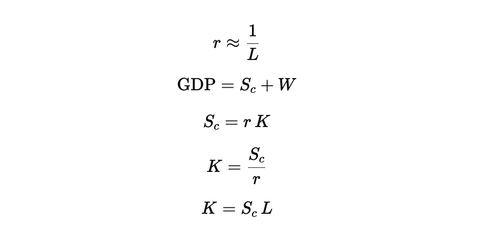
The cost of the slave (purchase price plus maintenance over the entire useful working life—that is, C + M*L, where C is the purchase price, M the annual maintenance cost, and L the duration of working life) constitutes the capital that makes the generation of profit possible. In the modern world, the equivalent would be the capital (K) required for the functioning of the economy. Here we must take into account that if r ≈ 1/L and Sc is the share of income that accrues to capital, then the amount of capital needed to sustain that relationship cannot be measured by summing up existing assets; it must instead be understood through the temporal scale defined by L. Capital (K) is not measured—it is inferred.

Accordingly, the calculation of K follows from considering the share of capital in GDP (GDP minus labor costs, which we denote Sc), divided by r (that is, by 1/L); in other words, Sc*L. The capital required to generate the observed return is thus the capital share of income multiplied by the length of working life.

The result is far greater than what one obtains by summing a country’s assets in the manner used by Piketty in his studies of capital, because in this framework capital includes the cost of raising, educating, and training workers, as well as all other conditions that make economic functioning possible. With a capital share of 40% of GDP, the resulting K—for an r of 4.5%—would amount to 12.5 times GDP. In the Roman example, the resulting K would be 7.5 times annual output (2,025 denarii for an annual output of 270). This means that in Rome capital represented a smaller proportion of income than today, but still one far larger than what emerges from attempts to “count” existing assets in a given economy.

I am fully aware that this is not the usual way of calculating the capital stock of an economy; yet it is the only way to account for everything that is actually required for production. The Roman slave example, in its simplicity, contains all the necessary elements. Here, the workforce is “capitalized” in an evident way through the right of ownership. The fact that, today, the relationship between worker and employer differs fundamentally—in legal, moral, and political terms—from that of a slave society should not obscure the structural point: in both cases, the relationship between capital and labour is organised in essentially the same way, as we have already suggested.

What changes is that part of the cost of “maintaining” the worker is now externalized—borne either by society as a whole (basic public services) or by the family that has raised and educated the worker. Excluding these elements from the measurement of capital explains the difference between the result of this approach (K = Sc*L) and that obtained by trying to quantify existing assets at a given moment. The two approaches do not measure the same thing: one measures the structural capacity to sustain labour; the other measures the ownership of assets.

In the end, this is only a hypothesis—an attempt to link that persistent mystery (the remarkable constancy of the return on capital) with something tangible: the duration of human life, or more specifically, the span of our working life. The return on capital is nothing more than the shadow that our lives cast upon the economy.